In my penultimate year of university, I joined Jump Trading for a six-month industry placement. I later returned for another two years. During that time, I worked on some of the most interesting problems in HFT infrastructure.

Around exchanges such as CME, NYSE, and NASDAQ, most of the easy latency wins are long gone. In many cases, the race is no longer at the application layer. It often comes down to Layer 2¹, and sometimes even Layer 1² optimisations. This means that even the tiny amount of latency introduced by queueing on one of these links can become a critical bottleneck.

One such L2 optimisation involves detecting and addressing packet queueing on a Layer 2 link. This project taught me a lesson that stuck: guessing where latency comes from never works. Guessing is the same as hoping.

“Hope is not a strategy.”

~Traditional SRE saying

Surely, devices track this already…

A natural starting point was switch-level counters. At Jump, we built a custom system to extract and process metrics from all our networking devices, which made this relatively straightforward. There’s a good PacketPushers podcast episode that covers this vendor-agnostic telemetry system in more detail.

In practice, though, things were less straightforward. On some devices, vendors simply did not support these counters. In other cases, switches required an OS upgrade. Sometimes vendors claimed the counters existed, but in reality, they did not. I opened plenty of TAC cases over this and became very good at going in circles.

Even in the rare cases where the counters were available, many of them lacked useful context. They did not expose L2 or L3 information such as source and destination IP and MAC addresses. At best, you could tell that queueing was happening on a link. You could not attribute it to a specific device or flow, which made debugging feel a bit like guessing with mildly better tooling³.

So I stopped relying on what the devices claimed and started working from first principles using only what we could see on the wire.

Detecting packet queueing using first principles

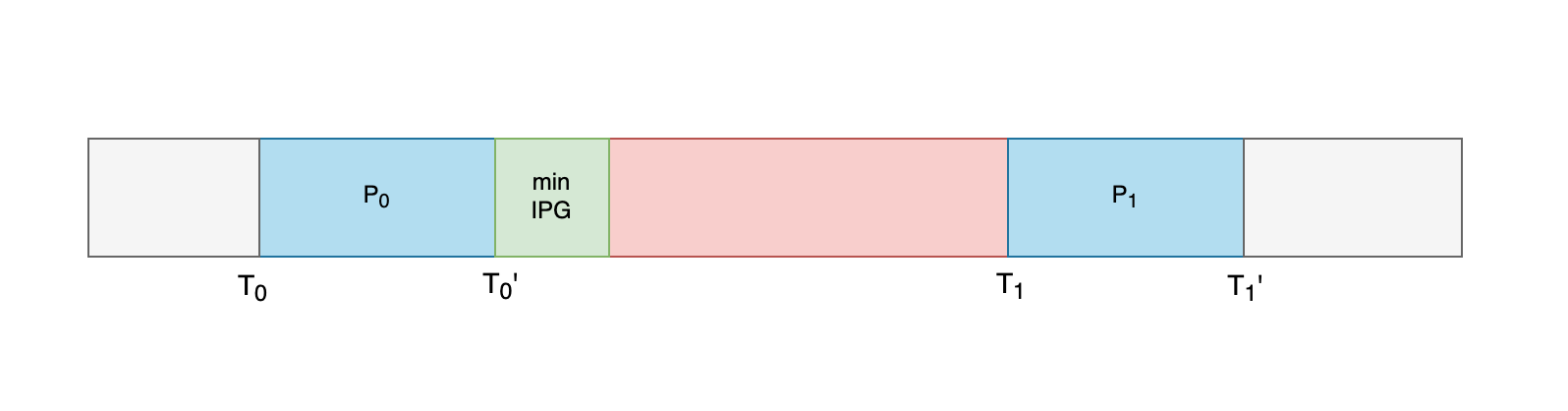
Consider two packets, $P_0$ and $P_1$. Suppose we observe their first-bit timestamps on the wire, i.e. the time at which the first bit of each packet is transmitted onto the link. We denote these timestamps by $T_0$ and $T_1$, respectively, and their on-wire lengths by $L_0$ and $L_1$.

Given the serialization delay of the link, $\alpha$ (time per byte), we can compute when each packet finishes transmitting:

So $T_0'$ represents the time at which $P_0$ has fully exited the link.

Ethernet links enforce a minimum interpacket gap, denoted $IPG_{min}$, which is the minimum required idle time between two consecutive packet transmissions.

This gives a strict physical constraint, illustrated in the figure above:

• After $P_0$ finishes transmitting at $T_0'$, the link must remain idle for at least $IPG_{min}$ before $P_1$ can begin transmitting.

So for packets observed on the wire, the following must hold⁴:

If packets arrive at the transmitter sporadically, the link will often sit idle, and we expect:

But if packets arrive faster than they can be transmitted, they must queue before transmission. In this case, the transmitter stays continuously busy and emits packets back-to-back at line rate. The observed gap then collapses toward the minimum allowed by the link:

A sustained collapse of the observable gap toward $IPG_{min}$ is indicative of queueing.

I needed really accurate timestamps

Up to this point, I had assumed that I could obtain precise ingress timestamps from every monitored link. In practice, that was a significant assumption.

Traffic from each link was observed through a passive tap, with each direction delivered to a capture NIC. The detector for an individual link compared timestamps from the same NIC clock.

Production monitoring, however, covered multiple links using multiple NICs. For example, observing two servers connected to the same switch meant observing two separate server-to-switch links, each with its own capture clock. Correlating events across those links required the clocks to agree at nanosecond scale.

Time synchronisation became the bottleneck almost immediately. NTP was not even in the conversation. PTP would get me closer, but it was not enough when nanoseconds mattered.

At that point, I needed to move into the world of hardware timestamping. Systems such as White Rabbit, originally developed at CERN and now used in finance, give an idea of what is possible when pushing the limits.

Fortunately, some really smart people had already built a very solid timestamping setup, so I did not have to worry about this at all! If you are interested, Networking at the speed of light provides a good overview of the kind of infrastructure involved.

Replacing hope with dashboards

I did not want this to die in PoC hell, so I ensured it could be used in practice.

The project began as a simple proof of concept using a collection of PCAPs. From there, it evolved into a system we could run in production. Capture NICs wrote traffic to PCAP files, which were then processed by a small Go binary.

Before applying the calculation, the binary normalised the raw timestamps and captured frame lengths for each type of capture hardware. MetaWatch and Arista devices, for example, used different timestamp reference points and frame-length conventions. This gave the binary the consistent $T_i$ and $L_i$ values assumed in the equations above.

Running the analysis in production also required a few configuration parameters⁵.

The first parameter was the link bandwidth ($B$), which determined the serialization delay $\alpha = 8/B$ when $B$ was measured in bits per second and packet lengths in bytes.

To make the system more robust, I introduced two additional parameters:

This defined the acceptable deviation from the minimum interpacket gap. In reality, links do not always behave perfectly, and the observed gap can deviate slightly from the theoretical minimum⁶.

This represented the number of consecutive interpacket gaps that had to remain close to the structural minimum before an event was flagged. It helped filter out noise and focus on sustained queueing rather than one-off anomalies.

For each pair of packets, the observed gap was:

We treated the packets as departing back-to-back when:

An event was flagged when this condition held for $n$ consecutive gaps, corresponding to $n+1$ packets.

The binary then emitted “likely queueing events” along with the associated source and destination IP and MAC addresses.

We could now attribute likely packet queueing

Attaching L2 and L3 context to these events turned out to be the most valuable feature.

The signal did not reveal the exact queue depth or how long an individual packet had waited. It showed sustained back-to-back departures and, with the L2 and L3 context attached, where queueing was likely occurring.

Instead of knowing only that a link had queued, we could now see which flows were involved. That was usually enough to trace the traffic back to a machine and start debugging.

It did not fix the queueing for us, but it told us where to start looking. That was a lot better than staring at a switch counter and hoping.

Notes